
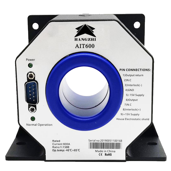
An accuracy error label compresses several behaviors into a number, even though an unchanged input can produce readings that shift with temperature or elapsed time. Interpreting precision starts with the relationship between the actual current and the indicated value, then examines what disturbs that relationship.
An accuracy-class assessment needs the applicable definitions and test conditions before a numerical limit becomes meaningful. Static deviations, changing signals and operation beyond the measuring range require different observations, each contributing a distinct part of the error analysis.
Attach the Accuracy Limit to Its Test Conditions
The DC accuracy limit of the Hangzhi AIT600-SG is 10 ppm at 25 ±10°C. That temperature interval and DC input condition belong with the figure whenever a high accuracy current sensor is assessed. The model also specifies a maximum linearity error of 2 ppm, describing a separate characteristic of its transfer relationship.
Linearity concerns how closely the output follows the intended relationship as input changes. A zero offset can shift the relationship without creating the same pattern as a deviation that varies across the range.
Recording readings at several known inputs makes those behaviors distinguishable; a single measurement point cannot describe the entire transfer characteristic. Repeated observations at each point can also separate persistent displacement from the scatter between successive readings.
The AIT600-SG has nominal ratings of ±600 A DC and 424 A AC RMS, with a measuring range of ±720 A. These values identify input conditions for the device. An accuracy-class label would additionally require the definitions of its classification scheme, so the individual ppm statements retain their own meanings rather than becoming an assumed certified class.
Trace Offset Through Temperature, Time and Supply
Zero offset appears as an indicated current when the actual input is zero. Its relative effect grows as the measured signal becomes smaller, because the same additive displacement occupies a larger fraction of that signal. A high precision current sensor therefore needs an offset description alongside its behavior at substantial input current.
For the AIT600-SG, the zero-offset limit at 25°C is 1 ppm, with user adjustment to zero available. Its maximum offset-temperature coefficient is 0.1 ppm/K, while maximum offset stability over time is 0.2 ppm/month. The specifications describe different influences on the baseline: a temperature change and an elapsed interval are separate variables in the investigation.
Supply-voltage interference is limited to 1 ppm/V for this model. Assessing that contribution requires the supply variation experienced by the device, just as a temperature coefficient requires a temperature difference.
A repeatable zero check can reveal a changed baseline, but identifying its cause requires the environmental and electrical conditions to be recorded. Changing one influence while holding the others steady gives the resulting difference a clearer physical interpretation.
A separate full-temperature zero-offset-current limit is ±5 µA. Combining that figure with ppm, ppm/K or ppm/month requires a common reference and defined operating changes. Their numerical magnitudes alone cannot be added into a defensible total error. they must first be converted to the same reference current, such as full scale or rated current, before their magnitudes can be compared.
Measure Dynamic Behavior with the Appropriate Criterion
A changing input adds a time dimension to the assessment. A frequency-response test examines how signal amplitude varies with frequency, whereas a step test follows the output after a defined input transition. For a high accuracy current sensor, these tests answer different questions about waveform reproduction. A slowly varying signal and a rapid transition can expose different limitations within the same measurement chain.
The AIT600-SG from Hangzhi specifies a −3 dB bandwidth from DC to 500 kHz. Its maximum response time to 90% of nominal DC current is 1 µs at an input slew rate of 100 A/µs. The amplitude criterion belongs to the bandwidth statement, while the percentage endpoint and input rate belong to the timed response.
An observed transition also depends on the applied waveform and the equipment receiving the secondary signal. Preserving those conditions makes a measured delay interpretable, and retaining the frequency-response criterion identifies the attenuation being assessed. Neither result extends the 10 ppm DC accuracy to all AC frequencies.
Check Loading and Recognize Loss of Proportional Output
Secondary loading participates in the operating conditions of a high precision current sensor. Within the same AIT series, the AIT1000-SG is specified here as the loading example: it lists a typical burden resistance of 1.5 Ω and a maximum of 3 Ω, subject to its burden curve.
The curve constrains the permissible loading rather than granting the maximum under every supply and current combination. A burden chosen without those conditions can invalidate the assumed relationship between primary input and secondary measurement.
This model has a nominal DC rating of ±1000 A and a measuring range of ±1200 A. Beyond the specified measuring range, overload operation leaves the zero-flux state; secondary current remains at its specified maximum, the output loses proportionality to primary current, and interlock pins 3 and 8 disconnect. Applying the normal conversion ratio to that saturated output would mask further changes in the actual input.
A measured deviation belongs to a defined input, reference quantity and operating state; temperature determines which stated limit can apply. For a high accuracy current sensor from Hangzhi, offset checks, dynamic tests and loading conditions then contribute identifiable evidence to the assessment.
A validity check identifies whether the conversion relationship still applies to the recorded output. Keeping each result connected to its conditions makes the precision judgment reproducible, including the point where an output ceases to represent current proportionally.
Practical Checklist for Assessing Accuracy
- Record the conditions with every reading: ambient temperature, supply voltage and its variation, burden resistance, input waveform and frequency, and the time since the last zero adjustment.
- Keep the 10 ppm DC accuracy, the 2 ppm linearity, the 1 ppm zero offset and the 1 ppm/V supply sensitivity attached to their own test conditions; do not add them into a single total without a common reference and a defined change in each influence.
- Convert the ±5 µA full-temperature zero-offset limit to the same reference current before comparing it with the ppm-based terms.
- Use a frequency-response test for attenuation and a step test for response time; neither extends the DC accuracy statement to all AC frequencies.
- Verify that the burden stays within the burden curve for the actual supply and current, not merely below the 3 Ω maximum.
- After an overload, confirm that the output still tracks the primary current proportionally; a saturated secondary output no longer represents the primary current, so the normal conversion ratio must not be applied.
